Neural Cover Selection for Image Steganography

This blog post is written as an overview and summary of our recent work Neural Cover Selection for image Steganography by Karl Chahine and Hyeji Kim (NeurIPS 2024). Our code can be found here.

Framework summary

Image steganography embeds secret bit strings within typical cover images, making them imperceptible to the naked eye yet retrievable through specific decoding techniques. The encoder takes as input a cover image \(\mathbf{x}\) and a secret message \(\mathbf{m}\), outputting a steganographic image \(\mathbf{s}\) that appears visually similar to the original \(\mathbf{x}\). The decoder then estimates the message \(\hat{\mathbf{m}}\) from \(\mathbf{s}\). The setup is shown below, where \(H\) and \(W\) denote the image dimensions and the payload \(B\) denotes the number of encoded bits per pixel (bpp).

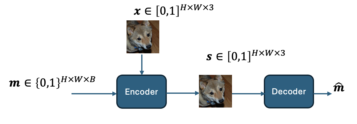
The effectiveness of steganography is significantly influenced by the choice of the cover image \(\mathbf{x}\), a process known as cover selection. Different images have varying capacities to conceal data without detectable alterations, making cover selection a critical factor in maintaining the reliability of the steganographic process.

Traditional methods for selecting cover images have three key limitations: (i) They rely on heuristic image metrics that lack a clear connection to steganographic effectiveness, often leading to suboptimal message hiding. (ii) These methods ignore the influence of the encoder-decoder pair on the cover image choice, focusing solely on image quality metrics. (iii) They are restricted to selecting from a fixed set of images, rather than generating one tailored to the steganographic task, limiting their ability to find the most suitable cover.

In this work, we introduce a novel, optimization-driven framework that combines pretrained generative models with steganographic encoder-decoder pairs. Our method guides the image generation process by incorporating a message recovery loss, thereby producing cover images that are optimally tailored for specific secret messages. We investigate the workings of the neural encoder and find it hides messages within low variance pixels, akin to the water-filling algorithm in parallel Gaussian channels. Interestingly, we observe that our cover selection framework increases these low variance spots, thus improving message concealment.

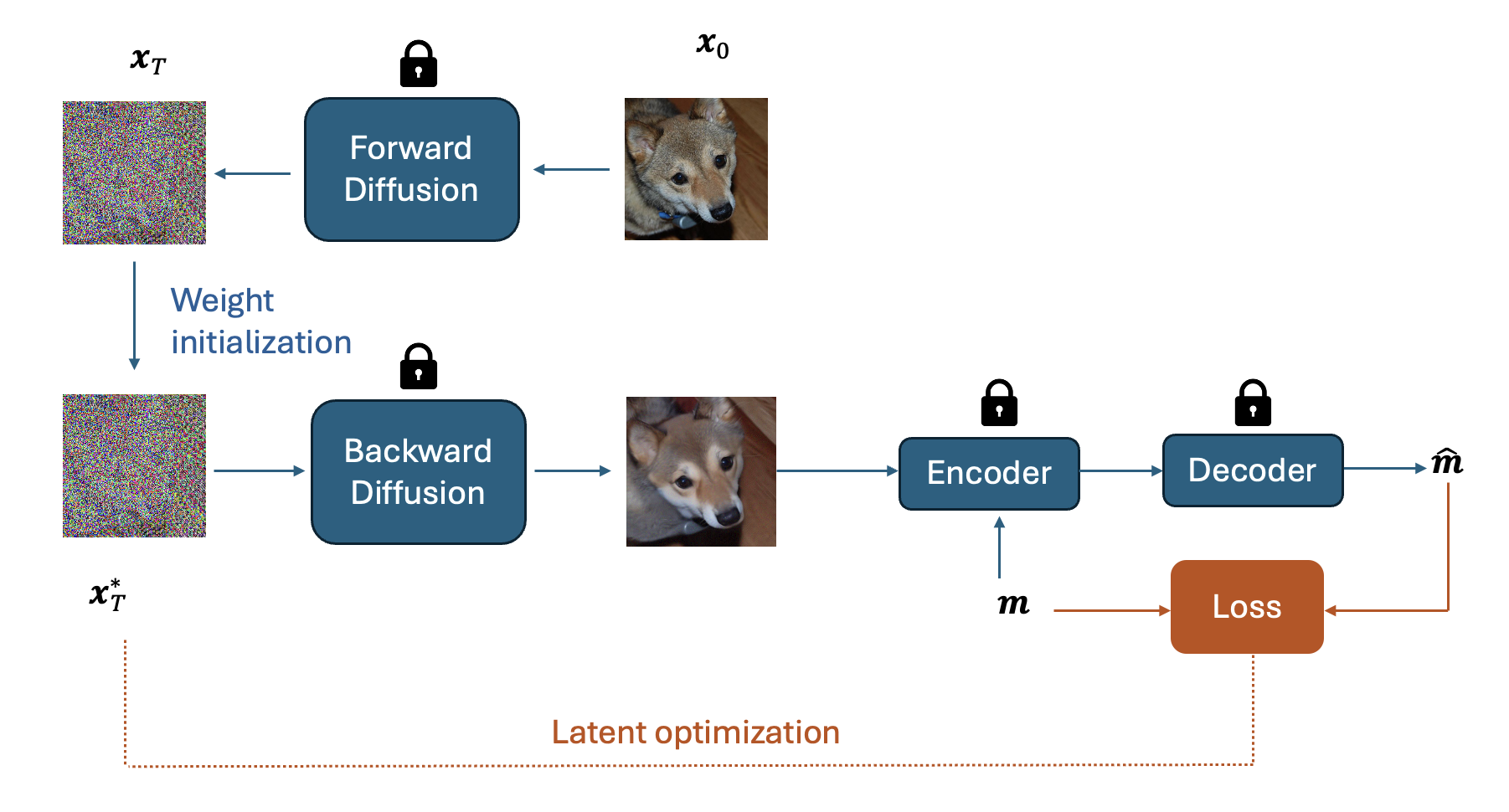
The DDIM cover-selection framework is illustrated below. The initial cover image \(\mathbf{x}_0\) (where the subscript denotes the diffusion step) goes through the forward diffusion process to get the latent \(\mathbf{x}_T\) after \(T\) steps. We optimize \(\mathbf{x}_T\) to minimize \(Loss(\mathbf{m}, \mathbf{\hat{m}})\). Specifically, \(\mathbf{x}_T\) goes through the backward diffusion process generating cover images that minimize the loss. We evaluate the gradients of the loss with respect to \(\mathbf{x}_T\) using backpropagation and use standard gradient based optimizers to get the optimal \(\mathbf{x}^*_T\) after some optimization steps. We use a pretrained DDIM, and a pretrained LISO, the state-of-the-art steganographic encoder and decoder from Chen et al. [2022]. The weights of the DDIM and the steganographic encoder-decoder are fixed throughout \(\mathbf{x}_T\)’s optimization process.

Performance results

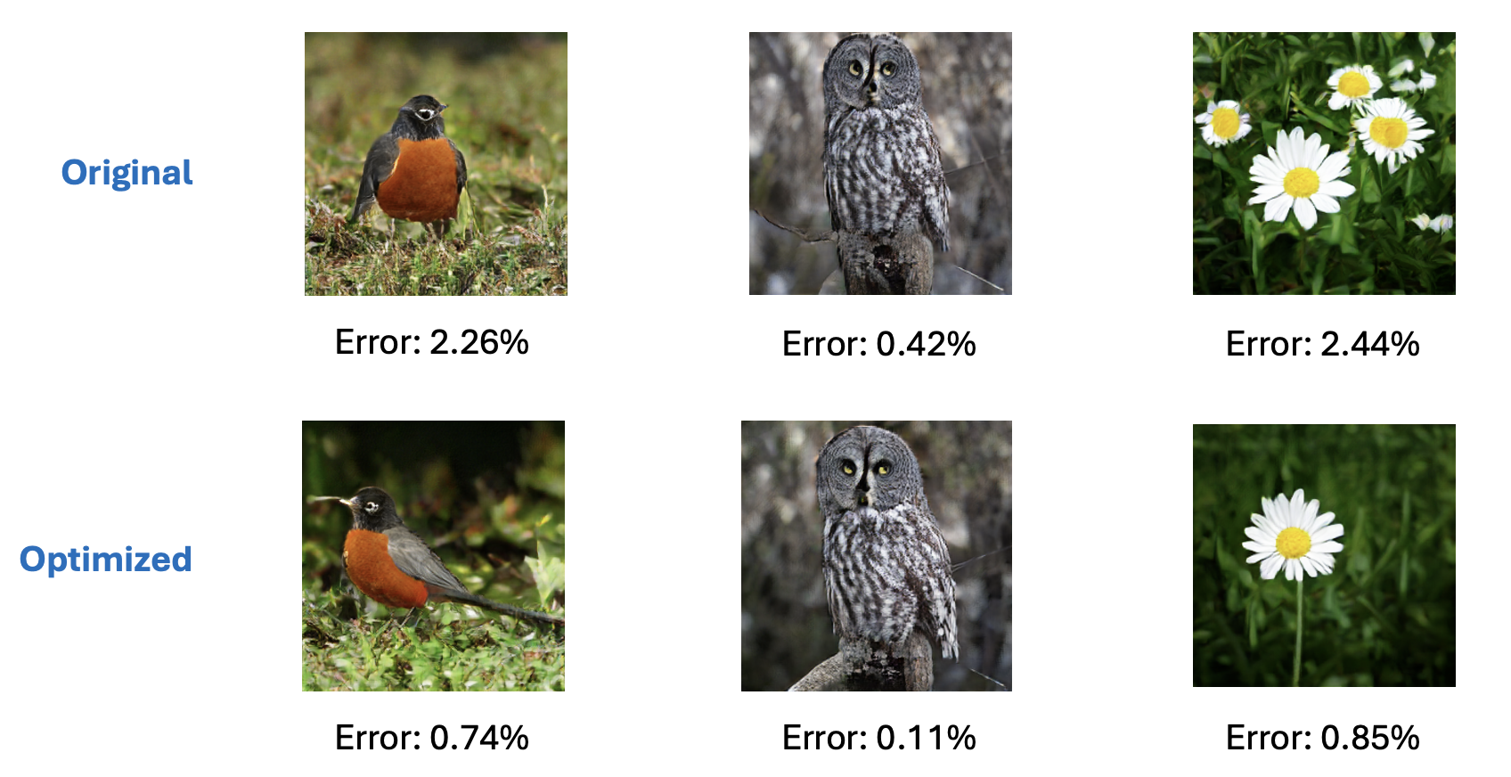
Below, we present randomly selected cover images alongside their message recovery errors, both before and after optimization. The observed error reduction post-optimization underscores the effectiveness of our framework.

Analysis

Encoding in low-variance pixels

We begin by investigating the underlying mechanism of the pretrained steganographic encoder. We hypothesize that the encoder preferentially hides messages in regions of low pixel variance. To test this hypothesis, we structure our analysis into two steps.

Step 1: variance analysis. Below, we illustrate the variance of each pixel position for the three color channels, calculated across a batch of images and normalized to a range between 0 and 1. The plot reveals significant disparities in variance, with certain regions displaying notably lower variance compared to others.

Step 2: residual computation. Using the same batch of images, we pass them through the steganographic encoder to obtain the corresponding steganographic images. We then compute the residuals by calculating the absolute difference between the cover and steganographic images and averaging these differences across the batch. This process yields three maps, one for each color channel, which are subsequently normalized to a range between 0 and 1. Those maps are plotted below.

we observe correlations between the variance and the magnitude of the residual values; where pixels with lower-variance tends to have higher residual magnitudes. To quantify this observation, we introduced a threshold value of 0.5. In the residual maps (from Step 2), locations exceeding this threshold are classified as “high-message regions” and assigned a value of 1. Conversely, locations in the variance maps (from Step 1) falling below this threshold are defined as “low-variance regions”, also set to 1. We discovered that 81.6% of the high-message regions coincide with low-variance pixels. This substantial overlap confirms our hypothesis and underscores the encoder’s tactic of utilizing low-variance areas to embed messages, which is a highly desired and natural behavior.

Analogy to waterfilling

To validate the findings presented above, we draw parallels between our analysis and the waterfilling problem for Gaussian channels. We conceptualize the process of hiding secret messages as transmitting information through \(N\) parallel communication channels, where \(N\) corresponds to the number of pixels in an image. In this analogy, each pixel operates as an individual communication link, with the secret message functioning as the signal to be hidden and later recovered. The cover image, which embeds the hidden message, serves as noise unknown to the decoder.

We consider a simple additive steganography scheme: \(s_i = x_i + \gamma_i m_i\), for \(i=1,2,...,N\), where \(N=H \times W \times 3\) is the image dimension, \(m_i\) indicates the \(i\)-th message to be embedded (either -1 or +1), \(\gamma_i\) its corresponding power, \(x_i\) and \(s_i\) represent the \(i\)-th element of the cover and steganographic images respectively. We assume a power constraint \(P\) that restricts the deviation between the cover and steganographic images: \(E \left[\sum_{i=1}^N (s_i - x_i)^2\right] \leq P\).

This formulation is similar to the waterfilling solution for \(N\) parallel Gaussian channels, where the objective is to distribute the total power \(P\) among the \(N\) channels so as to maximize the capacity \(C\), which is maximum rate at which information can be reliably transmitted over a channel, defined as: \(C = \sum_{i=1}^{N} \log_2\left(1 + \frac{\gamma_i^2}{\sigma_i^2}\right)\), where \(\sigma_i^2\) is the variance of \(x_i\). The problem can be formulated as a constrained optimization problem, where the optimal power allocation is given by \(\gamma_i^2 = \left(\frac{1}{\lambda \ln(2)} - \sigma_i^2\right)^+\), where \((x)^+ = \text{max}(x, 0)\) and \(\lambda\) is chosen to satisfy the power constraint.

We calculate \(\{\gamma_i^2\}_{i=1}^{3 \times H \times W}\) using a batch of images, and find the optimized \(\{\gamma_i^2\}_{i=1}^{3 \times H \times W}\) using the approach described above. We plot the \(\gamma_i\)’s for each color channel below.

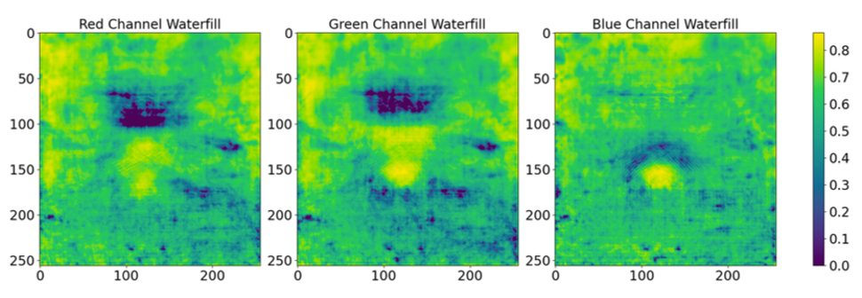
We observe a degree of similarity with the prior figure showing the residuals. To quantitatively assess this resemblance across color channels, we quantize the three matrices by setting values greater than 0.5 to 1 and values less than 0.5 to 0. For each channel, the similarity is calculated using the equation \(\frac{\sum_{i,j} \mathbf{1}(\textbf{W}^{(k)}_{ij} = \mathbf{R}^{(k)}_{ij})}{256 \times 256}\), where \(\textbf{W}_{ij}^{(k)}\) and \(\textbf{R}_{ij}^{(k)}\) are the \((i,j)\)-th pixels of the quantized waterfilling and residual matrices, respectively, for the channel \(k\). The computed similarity scores are 81.8% for red, 65.5% for green, and 74.9% for blue, revealing varying degrees of resemblance with the waterfilling strategy across the color channels. The variation underscores that the waterfilling strategy is implemented more effectively in some channels than in others.

Impact of cover selection

A natural question becomes: what is the cover selection optimization doing? We plot the variance maps of the optimized cover images below.

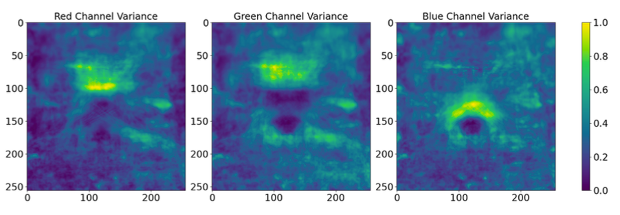
We notice that the number of low variance spots significantly increased as compared to the non-optimized images, meaning that the encoder has more freedom in encoding the secret message. Quantitatively, we find that 92.4% of the identified high-message positions are encoded in low-variance pixels, as compared to 81.6% before optimization. Given that the encoder preferentially embeds data in these low variance areas, this increase provides greater flexibility for data embedding, thereby explaining the performance gains observed in our framework.

For a deeper understanding and further details, we encourage you to review our research paper.