Distributed Source Coding
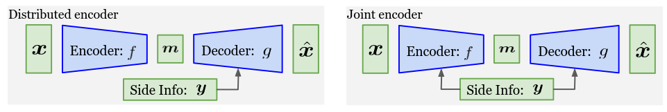
Distributed source coding (DSC) refers to the task of compressing multiple correlated data sources that are encoded separately but decoded jointly. A canonical example is a pair of images captured by stereo cameras on two different devices. The images represent correlated sources that must be compressed independently on each camera, but a joint decoder can exploit correlations between them for better reconstruction quality. In their groundbreaking 1973 paper, Slepian and Wolf proved the surprising result that separate encoding of correlated sources can asymptotically achieve the same compression rate as joint encoding. This defied conventional wisdom at the time, which held that joint encoding would always be superior since the encoder could directly exploit correlations between the sources. However, the Slepian-Wolf theorem showed that distributed compression is theoretically just as efficient.
Motivating Example
The curious reader might enjoy this simple example (repeated here from our paper) for intuition on the Slepian-Wolf theorem. Let \(\boldsymbol{x}\) and \(\boldsymbol{y}\) be uniformly random \(3\)-bit sources that differ by at most one bit. Clearly, losslessly compressing \(\boldsymbol{x}\) requires \(3\) bits. However, if \(\boldsymbol{y}\) is known to both encoder and decoder, then \(\boldsymbol{x}\) can be transmitted using \(2\) bits instead. This is because the encoder can send the difference between \(\boldsymbol{x}\) and \(\boldsymbol{y}\), which is uniform in \(\{000,001,010,100\}\). Thus, joint compression uses \(2\) bits.
Now, if the side information \(\boldsymbol{y}\) is available only at the decoder, Slepian-Wolf theorem suggests that the encoder can still transmit \(\boldsymbol{x}\) using only \(2\) bits. How could this be possible? The key idea is to group \(8\) possible values of \(\boldsymbol{x}\) into \(4\) bins, each containing two bit-strings with maximal Hamming distance: \(\mathcal{B}_0 = \{000,111\}\), \(\mathcal{B}_1 = \{001,110\}\), \(\mathcal{B}_2 = \{010,101\}\), \(\mathcal{B}_3 = \{011,100\}\). Then the encoder simply transmits the bin index \(\boldsymbol{m} \in \{0,1,2,3\}\) for the bin containing \(\boldsymbol{x}\). The decoder can produce the reconstruction \(\boldsymbol{\hat x}\) based on the bin index \(\boldsymbol{m}\) and \(\boldsymbol{y}\); precisely, \(\boldsymbol{\hat x} = \arg\max_{\boldsymbol{x} \in \mathcal{B}_{\boldsymbol{m}}} P(\boldsymbol{x}|\boldsymbol{y})\). Since \(\boldsymbol{x}\) and \(\boldsymbol{y}\) are off by at most one bit and the Hamming distance between the bit strings in each bin is \(3\), the decoder can recover \(\boldsymbol{x}\) without error given \(\boldsymbol{y}\). In other words, the side information allows the decoder to correctly choose between the two candidates in the bin specified by the encoder. DIstributed Coding Using Syndromes (DISCUS) introduces a constructive scheme for the distributed coding of correlated i.i.d. Bernoulli sources.
Although the Slepian-Wolf theorem is stated for the lossless case, it can readily extended to lossy distributed compression by first quantizing the source, then applying Slepian-Wolf coding. This scheme is known as Wyner-Ziv coding. As opposed to previous work, which assume i.i.d. data sources, we use deep learning in the DSC setting to learn to compress data with complex correlations, such as images.
Background: Evidence Lower Bound (ELBO) and VQ-VAE
The Vector Quantized Variational Auto-Encoder (VQ-VAE) is an architecture with discrete latents; it is trained on an objective modified from ELBO:
\[\log p(\boldsymbol{x}) \ge \text{ELBO}(\boldsymbol{x}) = \underbrace{\mathbb{E}_{q(\boldsymbol{z}\mid\boldsymbol{x})}\left[\log p(\boldsymbol{x}\mid\boldsymbol{z})\right]}_{\text{distortion}} - \underbrace{D_{KL}\left(q(\boldsymbol{z}\mid\boldsymbol{x}) \;\|\; p(\boldsymbol{z})\right)}_{\text{rate}}\]The evidence \(\log p(\boldsymbol{x})\) is lower bounded by term which measures the reconstruction loss (distortion) and a second term which regularizes the latent space (rate). Here \(p(\boldsymbol{x})\) represents the data distribution, \(p(\boldsymbol{z})\) is the distribution of the latent variable, and \(q(\boldsymbol{z}\mid\boldsymbol{x})\) and \(p(\boldsymbol{x}\mid\boldsymbol{z})\) represent the encoder and decoder, respectively. Two common assumptions are that (1) \(p(\boldsymbol{x}\mid\boldsymbol{z})\) is Gaussian, in which case the distortion term simplifies to an MSE loss term, and (2) \(p(\boldsymbol{z}) = \mathcal{N}(\boldsymbol{0}, \boldsymbol{I})\).
The learning objective proposed in the VQ-VAE paper modifies ELBO by assuming MSE loss for the distortion term, and assuming \(p(\boldsymbol{z})\) is uniform such that the rate term is constant (and can therefore be ignored). A commitment loss term is added to penalize the cost of committing to specific codebook vectors. As suggested in the VQ-VAE paper, the codebook can be updated via moving averages instead of including an additional loss term for vector quantization. The VQ-VAE loss is given by
\[\mathcal{L}(\boldsymbol{x}; f,g,\mathcal{C}) = \|g(c_\boldsymbol{m}) - \boldsymbol{x}\|^2 + \beta\|f(\boldsymbol{x}) - \texttt{stop_grad}(e_{\boldsymbol{m}})\|^2\]where \(f\) and \(g\) are the encoder and decoder networks, respectively, \(e_{\boldsymbol{m}}\) is the embedding vector of codebook index \(\boldsymbol{m}\), and \(c_{\boldsymbol{m}} = \arg\min_{c \in \mathcal{C}} \|c - f(\boldsymbol{x})\|.\)
Our Method: Distributed Evidence Lower Bound (dELBO)
One of our primary contributions is a modification of ELBO to the DSC setting. Under this setting, the decoder has access to \(\boldsymbol{y}\) and therefore we are more interested in bounding \(\log p(\boldsymbol{x}\mid\boldsymbol{y})\) rather than \(\log p(\boldsymbol{x})\). Here, we present a modified version of ELBO, called dELBO (full details and proof are provided in our paper):
\[\log p(\boldsymbol{x}\mid\boldsymbol{y}) \ge \text{dELBO}(\boldsymbol{x},\boldsymbol{y}) \triangleq \mathbb{E}_{q(\boldsymbol{z}\mid\boldsymbol{x})}\left[\log p(\boldsymbol{x}\mid\boldsymbol{y},\boldsymbol{z})\right] - D_{KL}\left(q(\boldsymbol{z}\mid\boldsymbol{x}) \;\|\; p(\boldsymbol{z})\right)\]Note that dELBO correctly reflects the distributed setting since the encoder \(q(\boldsymbol{z}\mid\boldsymbol{x})\) does not depend on the side information \boldsymbol{y}, but the decoder \(p(\boldsymbol{x}\mid\boldsymbol{y},\boldsymbol{z})\) does. We use dELBO to justify an alteration to the VQ-VAE training objective; the final training objective we use is given below:
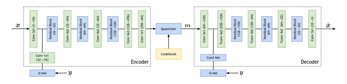
\[\mathcal{L}_{\text{dELBO}}(\boldsymbol{x}, \boldsymbol{y}; f,g,\mathcal{C}) = \|g(c_\boldsymbol{m}; \boldsymbol{y}) - \boldsymbol{x}\|^2 + \beta\|f(\boldsymbol{x}) - \texttt{stop_grad}(e_{\boldsymbol{m}})\|^2\]Again, the decoder network \(g\) is allowed to utilize the side information, but the encoder \(f\) cannot. The following figure illustrates our architecture for the joint setting; when training in the distributed setting, we remove the side information network (SI Net) and the \(1 \times 1\) convolution.
We trained our VQ-VAE architecture end-to-end on our \(\mathcal{L}_{\text{dELBO}}\) objective, and share some of our highlighted results and findings.
Results
Role of the Side Information
Even with the \(\mathcal{L}_{\text{dELBO}}\) objective and providing the decoder with side information, it is entirely possible that the VQ-VAE can learn to ignore the side information and instead just focus on learning to compress \(\boldsymbol{x}\). As a sanity check, we attempt the reconstruction of an image from the CelebA dataset when the decoder is given correct, incorrect, and random side information. Specifically, we divide the image into two halves, where the bottom half is the side information and the top half is the information we seek to compressed. In the below image, we show the reconstruction quality of the top half of the image given the bottom half as side information.
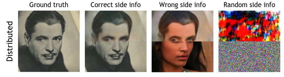
Providing the incorrect side information can affect the reconstruction by changing the color; providing random side information clearly confuses the decoder so that the reconstruction is distorted beyond recognition. One technical challenge of our neural DSC setup is that an adversary with access to the decoder could manipulate the final reconstruction by changing the side information. Such an adversary could lessen the quality of the reconstruction, or could distort the image to change the overall semantics.
Rate-Distortion Curves
The following figure highlights the rate-distortion trade-off between our and other methods. The figure on the right is trained with a modified \(\mathcal{L}_{\text{dELBO}}\) objective which minimizes the MS-SSIM metric rather than the MSE (PSNR).

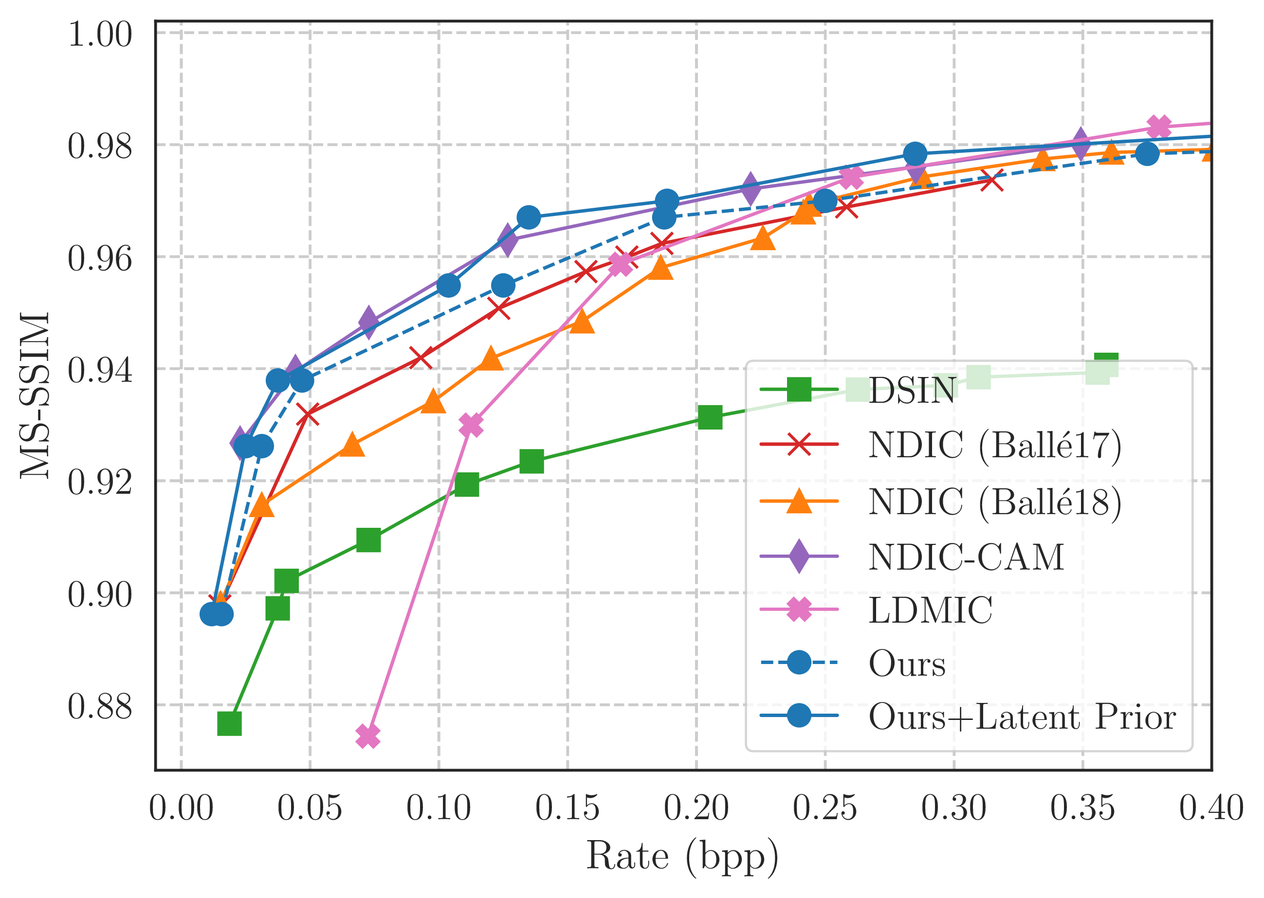
Through the use of a latent prior model, we can achieve a lower rate for a fixed distortion value. More specifically, we train an auto-regressive transformer model to learn \(p(\boldsymbol{z})\), and use arithmetic coding to compress with fewer bits. With the latent prior model, we are able to match the performance of the SOTA baseline (NDIC-CAM) on MS-SSIM, and outperform all baselines on PSNR.
Additional experiments in our paper compare our distributed setting with the joint setting (side information is available at the encoder), demonstrate the viability of neural DSC for gradient communication, and compare our learned approach with non-learning baselines on i.i.d. data. All of our code is available on GitHub
References
Neural Distributed Source Coding, Jay Whang, Alliot Nagle, Anish Acharya, Hyeji Kim, Alexandros G. Dimakis. IEEE Journal on Selected Areas in Information Theory, June 2024.
Noiseless coding of correlated information sources, David Slepian, Jack Wolf. IEEE Transactions on Information Theory, July 1973.
Distributed source coding using syndromes (DISCUS): design and construction, S. Sandeep Pradhan, Kannan Ramchandran. Proceedings DCC’99 Data Compression Conference, March 1999.
The rate-distortion function for source coding with side information at the decoder, Aaron Wyner, Jacob Ziv. IEEE Transactions on Information Theory, January 1976.
Neural discrete representation learning, Aaron van den Oord, Oriol Vinyals, Koray Kavukcuoglu. 31st Conference on Neural Information Processing Systems, December 2017.