Decoding convolutional codes

The Viterbi algorithm exactly computes the Maximum Likelihood (ML) estimate of the transmitted convolutional codeword over an AWGN (additive white Gaussian noise) channel. The algorithm is an early instance of dynamic programming. Although statistically this cannot be improved upon, we train a deep neural network to re-discover a Viterbi-like algorithm that matches the ML performance. Here the emphasis is on “algorithm”; we want to learn a decoder that can be readily applied “as is”, beyond block lengths it was trained on. In particular, a trained decoder is not considered an algorithm, if it only works for a fixed block length.

The purpose of this exercise is twofold. First, our ultimate goal is the discovery of new codes (encoders and decoders). Demonstrating that deep learning can reproduce an important class of decoders (for existing codes) is a necessary intermediate step. Next, we might want to adapt the decoder to handle deviations from the AWGN channel model or handle additional constraints on the decoder, such as low latency. Deep learning could provide the needed flexibility which Viterbi algorithm is not equipped with.

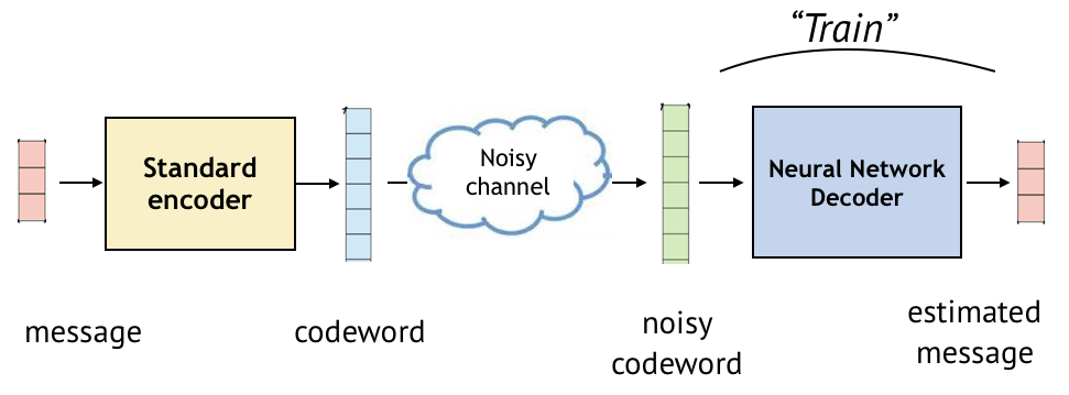
Consider communicating a message over a noisy channel. This communication system has an encoder that maps messages (e.g., bit sequences) to codewords, typically of longer lengths, and a decoder that maps noisy codewords to the estimate of messages. This is illustrated below.

Among the variety of existing codes, we start with a simple family of codes known as covolutional codes. Several properties make them ideal for our experiement.

These codes are practical (used in satellite communication) and form the building block of Turbo codes which are used for cellular communications.
With sufficient memory, the codes achieve performance close to the fundamental limit.
The recurrent nature of sequential encoding aligns very well with a class of deep learning architectures known as Recurrent Neural Networks (RNN).
Well-known decoders exist for these codes. For convolutional codes, maximum likelihood decoder on AWGN channels is the Viterbi decoder, which is an instance of dynamic programming.

Convolutional codes

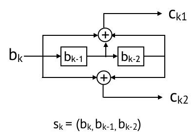
Convolutional codes were introduced in 1955 by Peter Elias. It uses short memory and connvolution operators to sequentially create coded bits. An example for a rate 1/2 convolutional code is shown below. This code maps b_k to (c_k1, c_k2), where the state is (b_k, b_k-1, b_k-2), and coded bits (c_k1, c_k2) are convolution (i.e., mod 2 sum) of the state bits.

Viterbi decoding

Around a decade after convolutional codes were introduced, in 1967, Andrew Viterbi discovered the so-called “Viterbi decoder”, which is a dynamic programming algorithm for finding the most likely sequence of hidden states given an observed sequence sampled from a hidden Markov model (HMM). Viterbi decoder can find the maximum likelihood message bit sequence b given the received signal y = c + n, in a computationally efficient manner. An overview of Viterbi decoding is below; a detailed walkthrough can be found here and here.

Convolutional codes are best illustrated via a state-transition diagram. The state diagram of the rate 1/2 convolutional code introduced above is as follows (figure credit). States are depicted as nodes. An arrow with (b_k/c_k) from s_k to s_k+1 represents a transition caused by b_k on s_k; coded bits ck are generated and next state is s_k+1.

Trellis diagram unrolls the transition across time. Let s₀, s₁, s₂, s₃ denote the state (00),(01),(10),(11). All possible transitions rare marked with arrows, where solid line implies input b_k is 0, and dashed line implies input b_k is 1. Coded bits b_k are accompanied with each arrow.

In the trellis diagram, for each transition, let L_k denote the likelihood, defined as the likelihood of observing y_k given the ground truth codeword is c_k (e.g., 00,01,10,11). We aim to find a path (sequence of arrows) that maximizes the sum of L_k for k=1 to K.

The high-level idea is as follows. Suppose we know the most likely path to get to state s_k (0,1,2,3) at time k and the the corresponding sum of L_k for k = 1 to K. Given this, we can compute the most likely path to get to state s_k+1 (0,1,2,3) at time k+1 as follows: we take max_{s_k in {0,1,2,3}} (Accumulated likelihood at s_k at time k + likelihood due to the transition from s_k to s_k +1). We record the path (input) as well as the updated likelihood sum. After going through this process until k reaches K, we find s_K that has the maximum accumulatd likelihood. The saved path to s_k is enough to find the most likely input sequence b.

Viterbi decoding as a neural network

It is known that recurrent neural networks can “in principle” implement any algorithm Siegelmann and Sontag, 1992. Indeed, in 1996, Wang and Wicker has shown that artificial neural networks with hand-picked coefficients can emulate the Viterbi decoder.

What is not clear, and challenging, is whether we can learn this decoder in a data-driven manner. We explain in this note how to train a neural network based decoder for convolutional codes. We will see that its reliability matches that of Viterbi algorithm, across various SNRs and code lengths. Full code can be accessed here.

Connection between sequential codes and RNNs

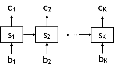
Below is an illustration of a sequential code that maps a message bit sequence b of length K to a codeword sequence c. The encoder first takes the first bit b₁, update the state s₁, and the generate coded bits c₁ based on the state s₁. The encoder then takes the second bit b₂, generate state s₂ based on (s₁, b₂), and then generate coded bits c₂. These mappings occur recurrently until the last coded bits c_k are generated. Each coded bits c_k (k=1, … K) is of length r when code rate is 1/r. For example, for code rate 1/2, c₁ is of length 2.

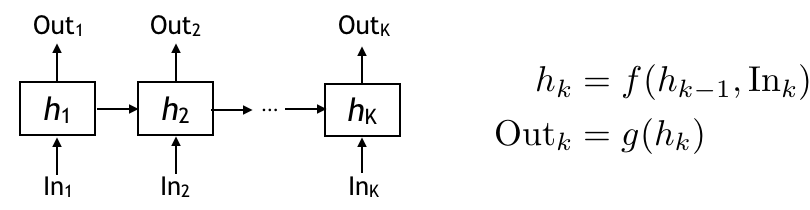
Recurrent Neural Network (RNN) is a neural architecture that’s well suited for sequential mappings with memory. There is a hidden state h evolving through time. The hidden state keeps information on the current and all the past inputs. The hidden state is updated as a function (f) of previous hidden state and the input at each time. The output then is another function (g) of the hidden state at time k. In RNN, these f and g are parametric functions. Depending on what parametric functions we choose, the RNN can be a vanilla RNN, or LSTM, or GRU. See here for a detailed description. Once we choose the parametric function, we then learn good parameters through training. So the RNN is a very natural match to a sequential encoder.

Learning an RNN decoder for convolutional codes

Training a decoder proceeds in four steps.

Step 1. Design a neural network architecture
Step 2. Choose an optimizer, a loss function, and an evaluation metric
Step 3. Generate training examples and train the model
Step 4. Test the trained model on various test examples

Step 1. Modelling the decoder as a RNN

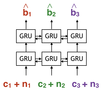
We model the decoder as a Bi-directional RNN that has a forward pass and a backward pass. this allows the decoder to estimate each bit based on the whole received sequence, instead of just the past ones. In particular, we use GRU; empirically, we see GRU and LSTM have similar performance. We also use two layers of Bi-GRU because the input to each 1st layer GRU cell is received coded bits, i.e., noise sequence n_k added to the k-th coded bits c_k. The output of each 2nd layer GRU cell is the estimate of b_k.

Here is an excerpt of python code that defines the decoder neural network. In this post, we introduce codes built on Keras library, for its simplicity, as a gentle introduction to deep learning programming for channel coding. The complete code and installation guides can be found here.

from keras import backend as K

import tensorflow as tf

from keras.layers import LSTM, GRU, SimpleRNN

step_of_history = 200 # Length of input message sequence  

code_rate = 2 # Two coded bits per one message bit

num_rx_layer = 2 # Two layers of GRU 

num_hunit_rnn_rx = 50 # Each GRU has 50 hidden units



noisy_codeword = Input(shape=(step_of_history, code_rate)) 

x = noisy_codeword

for layer in range(num_rx_layer):

   x = Bidirectional(GRU(units=num_hunit_rnn_rx, 

          activation='tanh',

          return_sequences=True))(x)

   x = BatchNormalization()(x)

x = TimeDistributed(Dense(1, activation='sigmoid'))(x)

predictions = x

model = Model(inputs=noisy_codeword, outputs=predictions)

Step 2. Supervised training - optimizer, loss, and evaluation metrics

We start with an RNN-based decoder model, whose parameters we learn in a supervised matter, using examples of (noisy codeword y, message b), via backpropagation. The goal of training is to learn a set of hyperparameters so that the decoder model generates an estimate of b from y that is closest to the ground truth b. Before we do the training, we choose optimizer , loss function, and evaluation metrics. Once these are chosen, training is made straightforward by deep learning tool kits. Summary of a model will show you how many parameters are in the decoder.

optimizer= keras.optimizers.adam(lr=learning_rate,clipnorm=1.)

#### custom evaluation metric: BER 

def errors(y_true, y_pred):

    ErrorTensor = K.not_equal(K.round(y_true), K.round(y_pred))

    return K.mean(tf.cast(ErrorTensor, tf.float32))



model.compile(optimizer=optimizer,loss='mean_squared_error', metrics=[errors])

print(model.summary())

Step 3. Supervised training

For training, we generate training examples, pairs of (noisy codeword, true message). To generate each example, we (i) generate a random bit sequence (of length step_of_history), (ii) generate convolutional coded bits using commpy, an open source, and (iii) add random noise of Signal-to-Noise Ratio SNR. Choosing the right parameters for step_of_history and SNR is critical in learning a reliable decoder. The variable k_test refers to how many bits in total will be generated.

#### Generate pairs of (noisy codwords, true message sequence)

noisy_codewords, true_messages, _ = generate_examples(k_test=k, step_of_history=200, SNR=0)

The actual training is done with one line of code.

#### Train using the pre-defined optimizer and loss function 

model.fit(x=noisy_codewords, y=true_messages, batch_size=train_batch_size,

                callbacks=[change_lr],

                epochs=num_epoch, validation_split=0.1)

Step 4. Test on various SNRs

We test the decoder on various SNRs, from 0 to 6dB.

TestSNRS = np.linspace(0, 6, 7, dtype = 'float32')

for idx in range(0,SNR_points):

    TestSNR = TestSNRS[idx] 

    noisy_codewords, true_messages, target = generate_examples(k_test=k_test,step_of_history=step_of_history,SNR=TestSNR) 

    estimated_message_bits = np.round(model.predict(noisy_codewords, batch_size=test_batch_size))

    ber = 1- sum(sum(estimated_message_bits == target))*\

           1.0/(target.shape[0] * target.shape[1] *target.shape[2]) # target: true messages reshaped 

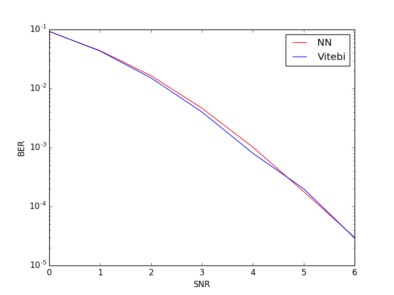
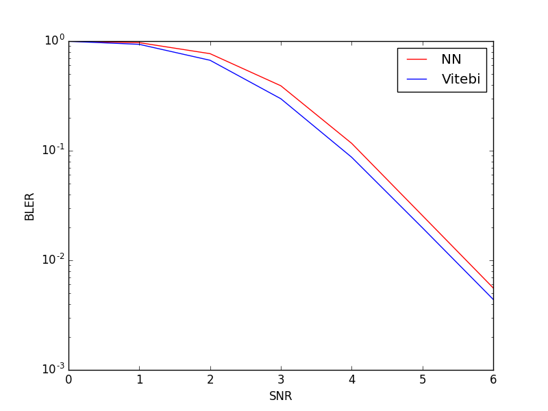
    print(ber)

We provide a MATLAB code that implements Viterbi decoding for convolutional codes for readers who would like to run Viterbi on their own. For SNRs 0 to 6, the Bit Error Rate (BER) and the Block Error Rate (BLER) of the learnt decoder and Viterbi decoder are comparable. Note that we trained the decoder at SNR 0dB, but it has learned to do an optimal decoding for SNR 0 to 6dB. We also look at generalization across different code lengths; we see that for arbitrary lenght of messages, the error probability of neural decoder is comparable with the one of Viterbi decoder.

References

Communication Algorithms via Deep Learning, Hyeji Kim, Yihan Jiang, Ranvir Rana, Sreeram Kannan, Sewoong Oh, Pramod Viswanath. ICLR 2018